9.1 Defining and Differentiating Parametric Equations
3 min read•january 24, 2023
Sumi Vora
Jed Quiaoit
Sumi Vora
Jed Quiaoit
AP Calculus AB/BC ♾️
279 resourcesSee Units
.png?alt=media&token=2e43c7f3-ca4e-495e-9b5b-11a043c870fc)
What is a Parametric Function?
Parametric functions are a set of related functions where x and y are independent from each other, but they are connected using the dummy variable t, which represents time. When we use the cartesian graph, we assume that we are moving along the x-axis in only one direction at a constant rate. However, parametric equations give us more freedom to manipulate horizontal motion.
A parametric equation would look something like this:
x(t) = t^2 - 1, y(t) = 3t
In this equation, your x-coordinate would be determined by t^2-1 and your y-coordinate would be determined by 3t. So, when t = 1, you would plot the point (0, 3). In a parametric function, t isn’t actually on the graph; we just use t as our constant so that our points are independent from one another.
There are several methods for calculating derivatives of real-valued functions, such as the limit definition, the power rule, the product rule, and the quotient rule. These methods can be extended to parametric functions, which are functions that depend on both a real variable and one or more parameters.
One way to extend these methods to parametric functions is to treat the parameters as constants and use the usual rules for differentiation. For example, if a parametric function is given by f(x,p) = px^2, where x is the real variable and p is the parameter, then the derivative with respect to x can be calculated using the power rule as df/dx = 2p*x.
However, our method for computing derivatives will actually be much simpler than the method above. Excited? 😄
Derivatives of Parametric Functions
Like we discussed earlier, a parametric function is still graphed in 2D on an xy-plane, so if we wanted to find the slope of the tangent line, we would still need to find dy/dx
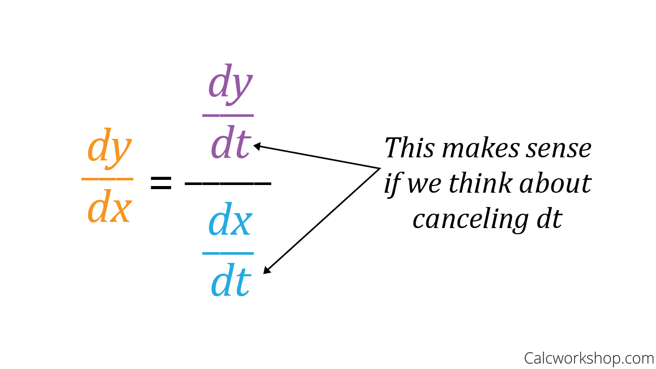
If we divide dx/dt and dy/dt, then dt will cancel out.
(dy/dt)/(dx/dt) = dy/dx
.png?alt=media&token=6aa39361-ae1a-4311-95ca-d1e78289129b)
*In the below example equation, it is t^2*
.png?alt=media&token=e97ef18e-f79d-45a3-a8da-565687ced852)
Still confused? Let's go into further detail.
This idea is known as the "parametric derivative" in calculus, often used to find the instantaneous rate of change of a parametric curve at a specific point. It is important to note that this method can only be used for parametric equations, where the curve is defined using a set of parametric equations in terms of a parameter, such as t.
To find the slope of the tangent line at a point on the curve, we first find the derivative of the x-coordinate function with respect to the parameter and the derivative of the y-coordinate function with respect to the parameter. These derivatives are denoted as dx/dt and dy/dt respectively. ⛰️
Then, at a specific point on the curve (x,y), the slope of the tangent line is found by taking the ratio of the derivative of the y-coordinate function with respect to the parameter (dy/dt) to the derivative of the x-coordinate function with respect to the parameter (dx/dt). This is the equation dy/dx = dy/dt / dx/dt!
It is important to note that the above equation is only valid if dx/dt is not equal to zero at the point of interest, as a vertical tangent line would not have a well-defined slope.

Source: Calcworkshop
Browse Study Guides By Unit
👑Unit 1 – Limits & Continuity
🤓Unit 2 – Fundamentals of Differentiation
🤙🏽Unit 3 – Composite, Implicit, & Inverse Functions
👀Unit 4 – Contextual Applications of Differentiation
✨Unit 5 – Analytical Applications of Differentiation
🔥Unit 6 – Integration & Accumulation of Change
💎Unit 7 – Differential Equations
🐶Unit 8 – Applications of Integration
🦖Unit 9 – Parametric Equations, Polar Coordinates, & Vector-Valued Functions (BC Only)
♾Unit 10 – Infinite Sequences & Series (BC Only)
🧐Multiple Choice Questions (MCQ)
✍️Free Response Questions (FRQ)
📆Big Reviews: Finals & Exam Prep

© 2023 Fiveable Inc. All rights reserved.