4.3 Introduction to Probability

5 min read•december 30, 2022

Kanya Shah

Aly Moosa

Jed Quiaoit

Kanya Shah

Aly Moosa

Jed Quiaoit

AP Statistics 📊

265 resources

See Units

💡 The big idea of this section and the rest of the math-y part of probability: The likelihood of a random event can be quantified!

That being said, we'll learn how to (1) calculate probabilities for events and their complements and (2) interpret probabilities for events. Not too daunting for an introductory dive into the basics of probability, huh? 🔐

Basic Probability Rules

A probability model is a mathematical representation of a chance process that is used to describe the likelihood of different outcomes occurring. It consists of two main components: a list of all possible outcomes and the probability of each outcome occurring.

The sample space is a list of all the possible outcomes of a chance process, such as flipping a coin or rolling a die. For example, the sample space for flipping a coin might be {heads, tails}, while the sample space for rolling a die might be {1, 2, 3, 4, 5, 6}.

Using this model, probabilities are usually expressed as fractions or decimals. For example, the probability of flipping heads when flipping a coin is 0.5, and the probability of rolling a 6 when rolling a die is 1/6.

A probability model is a description of some chance process that is made up of two portions: a list of all possible outcomes and the probability for each outcome. The list of all possible outcomes is called a sample space.

Rule 1: Equally Likely Probability

If all outcomes in a sample space are equally likely, the probability that event A occurs can be calculated by dividing the number of outcomes in event A by the total number of outcomes in the sample space. This is known as the classical definition of probability. 🟰

P(A) = number of outcomes in event A / total number of outcomes in the sample space.

For example, if we have a sample space of 6 outcomes (such as rolling a die), and event A consists of 3 of those outcomes (such as rolling a 1, 2, or 3), the probability of event A occurring would be 3/6, or 0.5. This is because there are 3 outcomes in event A, and there are a total of 6 outcomes in the sample space, so the probability of event A occurring is 3/6.

Rule 2: 0 Probability 1

Probabilities are always expressed as numbers between 0 and 1, inclusive, with a probability of 0 indicating that an event is impossible, a probability of 1 indicating that an event is certain to occur, and probabilities between 0 and 1 indicating that an event is possible but not certain.

For example, the probability of flipping heads when flipping a coin is 0.5, the probability of rolling a 6 when rolling a die is 1/6, and the probability of drawing an ace from a deck of cards is 4/52. These probabilities all fall between 0 and 1, indicating that these events are possible but not certain to occur.

When you do your math, getting probability values like -0.82 and 1.63 is an instant red flag! The good thing with this rule is that you can immediately sense something's wrong should you get such answers and immediately troubleshoot. 🚩

Rule 3: P(all outcomes) 1!

All possible outcomes MUST add up to 1. That's right! The probabilities of all possible outcomes in a sample space add up to 1. This is because the probability of an event occurring is a measure of the likelihood of that event occurring, and the probability of all possible events occurring must be 1 (since one of those events must occur).

For example, consider the probability of rolling a die. There are six possible outcomes (rolling a 1, 2, 3, 4, 5, or 6), and the probability of each outcome occurring is 1/6. If we add up the probabilities of all six outcomes, we get:

1/6 + 1/6 + 1/6 + 1/6 + 1/6 + 1/6 = 6/6 = 1

This demonstrates that the probabilities of all possible outcomes (rolling a 1, 2, 3, 4, 5, or 6) add up to 1, as expected. ➕

Rule 4: Complements

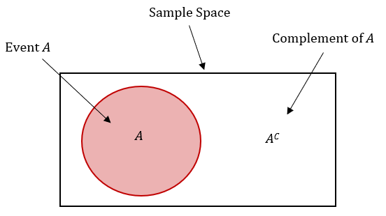
The probability of the complement of an event (also known as the inverse or opposite of an event) is equal to 1 minus the probability of the event occurring. This is because the probability of an event occurring and the probability of the event not occurring must add up to 1, since one of those two events must occur. ❌

Source: eCampus Ontario

For example, consider the probability of flipping heads when flipping a coin. The probability of flipping heads is 0.5, so the probability of flipping tails (which is the complement of flipping heads) is 1 - 0.5 = 0.5. Similarly, if the probability of rolling a 6 when rolling a die is 1/6, the probability of rolling any number other than a 6 (which is the complement of rolling a 6) is 1 - 1/6 = 5/6.

The College Board sometimes refers to the complement as E' or E^c (i.e. not E) = 1 - P(E). You'll most likely have to use this rule when problems ask for probability values mentioninig "at least ___" or "at most ___."

As you go through more sections, we'll add onto this growing list of probability rules. 😉

Probabilities and Context

Be sure to know how to interpret the probability you calculate. Remember to use words involving context!

Example

A company that manufactures car parts wants to understand the quality of their production process. To do this, they decide to sample a random selection of 100 car parts and test them for defects. The results of the testing show that 20 parts are defective and 80 parts are non-defective.

Based on the results of the testing, the company makes the following conclusions:

The probability that a randomly selected car part is defective is 20%.
The probability that a randomly selected car part is non-defective is 80%.
There is a 20% chance that a randomly selected car part will be defective.
There is an 80% chance that a randomly selected car part will be non-defective.

Write a brief summary explaining the company's conclusions and the statistical evidence that supports them.

Answer

The company concludes that the probability that a randomly selected car part is defective is 20%, and that the probability that a randomly selected car part is non-defective is 80%, based on the statistical evidence provided in the results of the testing. The company also concludes that there is a 20% chance that a randomly selected car part will be defective, and an 80% chance that a randomly selected car part will be non-defective.

The statistical evidence that supports these conclusions is the fact that 20 out of 100 car parts were defective, and 80 out of 100 car parts were non-defective. This means that the probability of a randomly selected car part being defective is 20/100, or 20%, and the probability of a randomly selected car part being non-defective is 80/100, or 80%.

🎥Watch: AP Stats - Probability Rules and Random Variables